Introduction

Complex models of atmospheric carbon dioxide concentration, that involve more than four or five parameters, are relatively useless in either hind-casting or predicting regardless of how well they may fit available data. So it is better to work with a model that only involves a few known critical physical parameters.

I propose dividing the earth’s surface into four zones; an emission zone and a sink zone in each hemisphere: and analyzing only the vertical flow in each. The net flow direction in the emission zones is up because the surface temperature is warmer than the air above it. In the sink zones the net flow direction is down because the surface is colder than the air above it

                                                                  The Model

The emission zones are mostly over water between 45S and 45N.  The sink zones are the remaining earths surface that includes the polar regions. The net vertical flow of CO2 in the emission zones is up, while it is down in the sink zones. Carbon dioxide in the atmosphere travels via jet streams from the upper atmosphere at emission zones to the upper atmosphere above the polar sink zones. The cold open waters nearer the poles are the ultimate sinks that are hardly ever a source. The Antarctic is mostly covered with snow and ice so it is not much of a source. The year round open waters that surround the land are an ultimate sink for CO2.

The emission zones are anywhere thunderstorms can form. Basically, energy from the sun evaporates surface water at near the atmospheric dew-point temperature. Evaporation is an endothermic process. Carbon dioxide is not only emitted via Henry’s law, but also because the evaporating water directly releases it into the atmosphere into which it evaporates.  Water vapor is lighter than air and rises dragging both air and CO2 with it. As it all rises, it gets less dense with fewer molecular collisions, thus, resulting in lower atmospheric temperatures. Each collision is transferring energy between molecules.  At the bottom of clouds, the air temperature approaches the dew-point temperature, and water vapor begins to condense. Condensation is an exothermic process that warms the air making it lighter so it rises faster. The warmed air drags water droplets and CO2 with it as it rises faster. The flow rate increases with elevation and can become fast enough to hold up golf ball size hail stones. While all this turbulent movement is occurring, cold rain-drops are absorbing CO2.  That rain delivers most of emitted CO2 back to the surface where it is available to be re-admitted.

However, a relatively small but significant fraction of CO2 goes out the top of thunderclouds to be transported by jet streams to polar sink zones.  The water that freezes releases its absorbed CO2, contributing to the fraction that eventually reaches a sink zone. Water, ice,and CO2   in the top of clouds radiates IR   upward to space. The clouds below absorb their downward IR to then be radiated to space. Air is relatively transparent to IR so it retains much of the energy it has gained from collisions with water vapor and CO2 molecules, while it travels to a sink zone.  That energy transfer mechanism with collisions is reduced in the upper atmosphere where density is lower.

At the sink zones, the surface receives little to no energy from the sun and it continually radiates to space. The day/night day is a year long. The surface is cooler than the air above it and cools the air. The air sinks and warms with more collisions to then be cooled by the radiating surface.

                                                      Testing the Model

Scripps has been measuring atmospheric CO2 concentrations in the Pacific since 1957. These data are published on their website; Sampling Station Records. They recorded data from ten sites ranging from South Pole at 90S to Alert, Canada at 82.3N. NOAA started measuring CO2 concentrations in the seventies and publish the results on their website, Four of their measuring sites are located at four Scripp’s sites; South Pole, Samoa, Mauna Loa, and Point Barrow. They consider these as “baseline” sites and also record meteorological changes. Other sources of relevant data are available at  WDCGG (World Data Centre for Greenhous Gases), Climate Explorer: Starting point, and ESRL : PSD : Monthly Mean Time series

Atmospheric concentrations of CO2 consist of both natural and anthropogenic emissions. Most anthropogenic emissions result from burning fossil fuels. Natural emissions result primarily from warming and evaporation of water both from oceans and land. Included in natural emissions are breathing of animals, forest fires. and decaying of biological materials. There are many more sources of natural emissions than there are for anthropogenic emissions and natural emission rates are much greater than emission rates resulting from burning fossil fuels.

Both natural and fossil fuel burning emission rates are changing with time. We have estimates of fossil fuel burning rates and we have been monitoring atmospheric concentrations of CO2 for several years. These data can be used to give us a better estimate of how the ratio of natural to fossil fuel burning emission rates change with time.

The two regions on earth that are consistently sinks for atmospheric CO2 are those regions north of 45 degrees North and south of 45 degrees South (Arctic and Antarctic). While the air is flowing downward from the upper atmosphere in all of the area, it is only being absorbed by the cold, open waters that are not covered with ice. The evidence for this fact is demonstrated by comparing the seasonal changes in atmospheric concentrations of CO2 with seasonal changes in sea-ice concentrations.

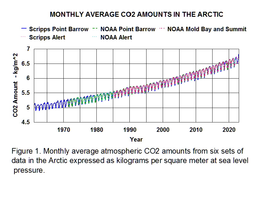
First, separate annual variations from year-to-year changes. The atmospheric concentrations of CO2 at measuring sites in each polar sink zone uniformly change with time. This uniformity is the result of the air being well mixed over the whole regions. This fact is graphically illustrated in Figure 1 by the very close agreement within six sets of data reported by two organizations from four different latitudes. The reported ppm concentrations   have been converted to kg/m^2 at sea level by multiplying by 44/28.8/1000000*1013*10.197. This is the estimated amount of CO2 in a square meter vertical column.

Sea-ice concentration north of the Arctic circle (66.5N) is shown in Figure 2.

                    Figure 2. Sea-ice concentrations in the Arctic north of 66.5N.

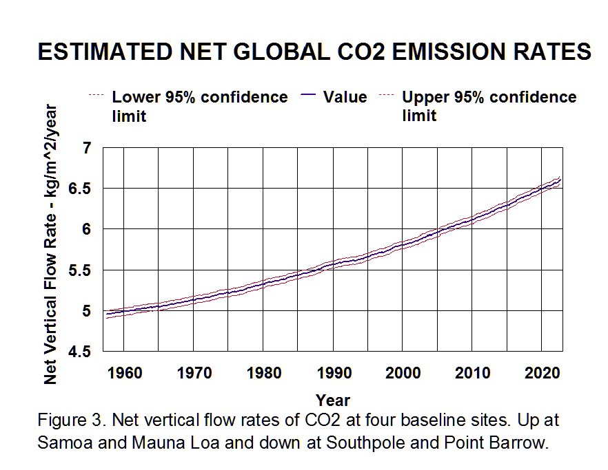
            The obvious difference between Figures 1 and 2 is the non-linear  long-term increase in CO2 concentration. Since the sink rate from the regions atmosphere is being controlled by the fraction of open sea water which varies within a year, the observed long-term change represents the input at the top of the Arctic regions atmosphere. A thirteen month running average of the atmospheric concentration represents these values.The input at TOA  Arctic is what is being delivered from the output at TOA of emission zones. Scripps reported  seasonally adjusted monthly averages in column 10 are statistically the same as the 13 month running averages and they have calculated these values for multiple sites in both emission and sink zones. Figure 3. shows  how well the values in two poles apart sink zones agree with values in the emission zones based on 13 month running averages.

 

            So  subtracting the column 10 value from the column 9 value of the Point Barrow Scripps data separates out the within-year variation for that site. The results of a simple regression of these results on the sea-ice concentrations is presented in Table 1.

                                              REGRESSION RESULTS

          Constant                                                                               -0.3239

          Standard Error of Y coefficient                                               0.0304

          R Squared                                                                            0.8980

          Number of Observations                                                              485

          Degrees of Freedom                                                                  484

          Coefficient for Sea-ice concentration                                      0.5159

          Standard Error of Coefficient                                                 0.0072

           f Statistic                                                                                   4170

Table 1. Simple regression of within year variation on sea-ice concentration north of Arctic Circle north of 66.5N.

          The line in Figure 3 may be considered a “global  signature” for natural emissions rates. . The slopes are not emission rates because  the values are year-long averages of monthly emission rates. The year-to-year differences are more like a second derivative with time (kg/m^2/year^2). Further evidence for this is that in the emission zones the rates are positive(up) while in the sink zones they are negative(down). When the slopes in Figure 3 are equal to zero the average of rates up in the emission zones are equal to the averages of rates down in the sink zones. These rates can be compared to estimated global emissions of CO2 from burning of fossil fuels as shown in Figure 4.

          The blue line is the reported values of annual global anthropological emissions divided by the surface of the earth in square meters. This is like assuming they are instantly distributed uniformly across the globe without any of the many sinks acting on the amount in the atmosphere. The values in Figure 3 are two orders of magnitude greater than the values in Figure 4. Considering all the sinks (mostly cold rain) that are absorbing anthropological emissions. it is practically impossible for these relatively small amounts to be contributing to atmospheric concentrations of CO2.

                                                  CONCLUSIONS

          1. The sink rate in the polar regions is being controlled by the amount of area of cold ocean water that is not covered by ice. In the Arctic winter, most of the ocean is covered by ice and CO2 concentrations  rise until the ice begins to melt. As the ice melts, the concentrations decrease reaching an annual minimum in September. There is no year-to-year accumulation. In the Antarctic, cold waters surround the land and freezing ice covers a much smaller fraction of the surface in the Antarctic winter so there is less CO2 concentration buildup each year.

          2.Comparing Figures 3 and 4 is very strong evidence that it is practically impossible for burning of fossil fuels to be adding any significant amount to the global atmospheric concentration of CO2. Carbon dioxide levels will continue to rise as more ocean water is evaporated and more CO2 is released to TOA . Stopping all fossil fuel burning will not have an effect on this process.

          3.  Nature has a very effective “net zero” in cold rain and cold polar open waters. There is no year-to-year atmospheric accumulation of either natural or anthropological emissions.            .